![]()
Neural Networks (Perceptrons) have interesting properties and applications - but would be best implemented on a parallel processing device such as a Field Programmable Gate Array (FPGA) I.C. (e.g. Alterra, Xilinx) than a computer CPU - however a standard PC can be used to demonstrate their behavior. The main attribute seems to be "pattern recognition" and the ability to be "trained" by repeated presentations of "lessons" that are muck like a school lesson. Therefore there is the following
| A Lesson Topic - to describe the general types of questions and answers | |
| The Lesson Question List - these are "stimulus" inputs to the Neural Network (NN) | |
| The Matching Lesson Answer List - these are the "targets" used to train the NN |
This "supervised training approach" is the easiest to start with as you can tell the actual performance - especially when it can take a long time to train the NN. This is unlike standard programming where software code exactly describes a series of processing steps. The NN is more random and based on an expectation that the NN performance will converge over time.
However it should be appreciated that the number of nodes ("neurons") in a NN is severely limited - a worm may have many more. So they don't show much "interpretive intelligence" other than to be able to remember a Lesson Topic. Some Topics with an internal pattern in the lessons may let a NN encode more efficiently, so that more memory may appear to be available than the number of nodes might suggest. This may be a useful property but the patterns may need to be simple.
The typical NN structure is similar to its biological "equivalent" and consists of an Input Layer of [I+1] of nodes that receive each input stimulus as a vector of numerical values [x0 ,x1 ,...,xI ]. Each input node has a Non Linear Transfer (NLT) function and several can be used. A linear transfer function won't work well it all as the NN would just be a matrix operation.
One common NLT function is the "Sigmod Function" defined as S{x} = 1 / [ 1 + exp{-x} ]. This function has an input range -inf < x <inf and an output bounded on 0 < S < 1. Once these values of S{x0 },...,S{xI } are computed the values are passed to a new "hidden" layer based on a series of scaling "Weights". These weights determine the behavior and may be derived iteratively. The NN can have any number of hidden layers but finally end up as a output vector following this "forward pass" procedure.
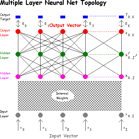
The task of training the NN is to find weight values (i.e. matrices of numbers) that produces an output that matches the target answer vector for each question to within some error tolerance Ek . Each layer can have different vector lengths but it may be easier to keep them the same depending on your software tools.
To appreciate the numerical effort assume there are 64 input nodes, 64 hidden and 64 outputs. The input to hidden layer weight matrix will now be 64 * 64 = 4096 in size with real numerical values. The hidden to output matrix will be the same size. Now consider 64 lessons - the weights do not update independently (not orthogonal) so updates to one weight term Wm,n need 64 repeats. Further, increasing the number of lessons reduces the memory performance and say 1,000 iterations may be needed for 64 lessons or 10,000 for 128 lessons. Since a computer has to perform these calculations sequentially the NN may be slow to train. (This is why a FPGA-CPU combination would be better).
(I remember an article in Scientific American about a decade back showing a simple 2 node, 3 layer net learning an XOR logic function. This took 10,000 iterations but I think there must have been a programming mistake somewhere!)
However, as an amateur experimenter I have found that you can get excellent training (very low Ek terms) even with random binary lessons (as long as one input is not expected to have two conflicting outputs!) and 8 nodes to 128 or so is doable on a standard PC and the performance degrades gracefully when the number of lessons is greater than about twice the number of nodes per layer. This can take a few minutes or an hour depending on the size. Four and Five layer NN work slightly better than 3 layer NNs but 10 layer NNs seem impractical.
If we consider the Interfaces = Layers -1, then a 4 layer NN will have 3 weight matrices each of which can be filled with random seed values prior to training. MATHCAD seems to have trouble with 3-D matrices so Initialize generates a sequence of weight matrices Wn,m cascaded according to the number of interfaces. I have shown these to be constrained between ±1 in this example.

ActionPotentials calculates the output values for each NN node based on the input vector x placed in the first column AP<0> .I have shown this progress from left to right with wm,n extracted from the composite matrix W.
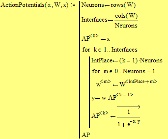
This uses the Sigmoid function and the output of all nodes are contained in AP.
I'll explain this later
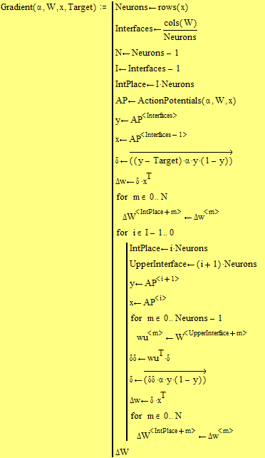
This is a "consensus based learning" approach rather than a competitive one - seems to work OK. The competitive training approach updates weights one lesson at a time so tends to show preference for first and last lessons. However if we average all gradients across all lessons (i.e. a consensus across all gradients) it then this effect disappears and the overall procedure "seems" to be more effective.
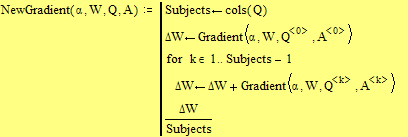
This is included for illustration based on a method of "steepest descent".

This MATHCAD file shows a small 8 node 4 layer NN trying to "recall" 64 random vectors as a memory task. It has had 1,500 iterations, the last 1,000th and 1,500th results as a percentage score per lesson.
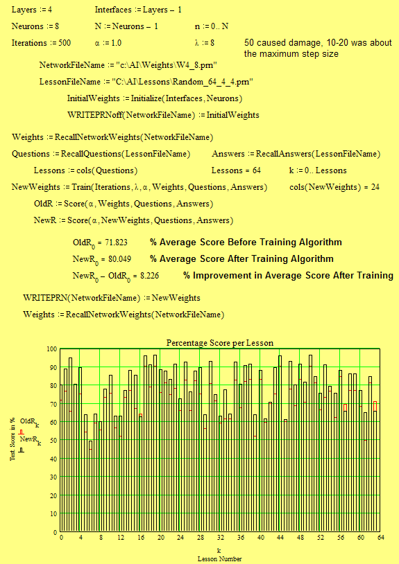
This examples places a high memory loading for the size of the NN so the average score is only 80%. This will continue to improve by smaller amounts over time. Alternatively, reducing the lesson size will result in scores around 99% although there may be some anomalous low scores.
Hopefully this web chapter introduces how Neural Nets work (simple ones) and how their behavior can be explored using relatively simple (but nice to use) tools such as MATHCAD. A complied program would be faster (MATLAB, C, etc) but a FPGA would be excellent.
![]()
Return to Artificial Intelligence
Return to Ian Scotts Technology Pages
© Ian R Scott 2007 - 2008