or return to A Component Universe
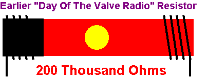
The earliest resistors consisted of various lengths of partly conducting wire, usually made from nichrome. The final resistance value was proportional to the length of the wire and inversely proportional to the wire diameter. Practical constraints limited both dimensions, and resistance values much greater than 1000 Ohms became impractical. This proved to be a problem, especially as Lee De Forest's triode component was a low current device, and circuits that could employ its amplification properties required much higher resistor values. The first applications used transformers, which provided a much higher AC impedance than the DC resistance of their windings, and so could overcome this limitation. Transformers of the time were hand wound and expensive, also very large. People soon reasoned that if they could use resistor-capacitor coupling, radio receivers could be smaller and less expensive.
The resistivity of nichrome is higher than that of copper, but carbon is higher still. Unfortunately carbon cannot be drawn into a wire. However it can be deposited on a ceramic tube, and mixed with insulating compounds to further increase its resistivity. This new invention resulted in the carbon deposition resistor.
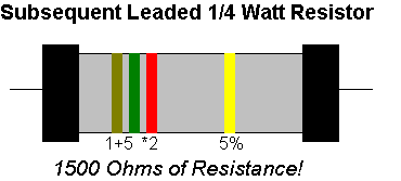
Early resistors were still physically large, and the resistance value could simply written on them. However, as improvements were made they became smaller and this approach became impractical. Two very useful concepts were introduced to overcome this, first the use of scientific number representation, and then the use of a color code that mapped numbers to colors.
Scientific notation represents numbers as a mantissa, usually two numbers, followed by an exponent. For example 1,2,5 in this notation would represent 1.2 * 105 = 120,000, similarly 5,6,2 represents 5.6 * 102 = 5,600.
This allowed a compact means to represent the actual component value. In early resistor components, accuracy was difficult, and 20 % variation was common. By the time the need for a compact format was needed, this had improved to 10 % accuracy. It therefore became apparent that resistor values should be fixed to certain fixed values, based on overlap caused by this tolerance. Since the magnitude of variation increased with the absolute value, it followed that these set values should follow a geometric scale, as opposed to equal increments.
This reasoning lead to the now standardized "E12" series, based on the following mantissa values.
1.0, 1.2, 1.5, 1.8, 2.2, 2.7, 3.3, 3.9, 4.7, 5.6, 6.8, 8.2
Today's improvement's in component manufacture have significantly reduced tolerances on all components, and E24 series etc are also included.
The color mapping to numbers was accepted to be
| 0 | 1 | 2 | 3 | 4 | 5 | 6 | 7 | 8 | 9 |
| Black | Brown | Red | Orange | Yellow | Green | Blue | Violet | Grey | White |
A tolerance band was also added, silver for 10 % and gold for 5 %, I guess that would be expected :)
These cylindrical resistors often used a spiral deposition of carbon to allow high values of resistance with less uncertainty caused by its composite mixing in insulating compounds. This created a parasitic inductance in series with its ohmic value. In addition, some parallel capacitance caused by the diameter of its end caps and the separating distance created a parallel capacitance.
In some RF circuits this was problematic, as the apparent AC resistance was different from its DC value. In the early 1930's, frequencies as high as 30 MHz were consider as "Ultra High Frequencies" or UHF. In the 1900's the definition of UHF migrated from 300 MHz and above. Today, UHF starts at 1 GHz.
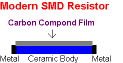
Leaded resistors of this form are completely unsuitable at these frequencies. In addition, modern manufacturing processes prefer to remove unnecessary steps, such as cutting unwanted lead length off after component placement on a PCB. The advent of Surface Mount Devices, or SMD avoided this, and such components were available as early as 1960 or so. The electronic industry avoided these for a long time, until about 1990 when many manufacturers invested in new plant equipment that could place and solder SMD. In today's electronics, SMD is the primary component choice.
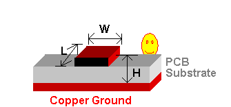
SMD resistors use a planar structure, although some can be cylindrical, referred to as "melf" resistors. They have the same basic construction, employing an insulating ceramic body with carbon deposition on the top side. Metal deposition at each end forms electrical terminations for the SMD resistor.
Once again, standardization of SMD sizes became introduced. These are defined in terms of length L and width W as follows
| L, .mm | 04 | 06 | 08 | 12 | 12 |
| W, .mm | 02 | 03 | 05 | 06 | 10 |
Note: these are given in imperial units of inches, for example 04 inches means 0.04 inches (2.05 mm), equally 12 inches means 0.12 inches (3.07 mm). These are connected as a four digit string where the first two digits refer to the component's length and the last two digits refer to the width. A size value of "0805" refers to a SMD component that has a length of 0.08 inches and a width of 0.05 inches.
These SMD resistors (equally capacitors and inductors) are directly mounted on a PCB.
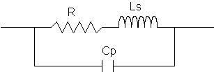
We can consider the resistor as a lossy transmission line as described by the following distributed circuit,
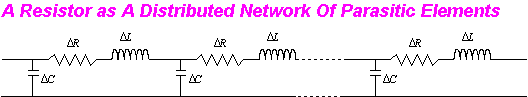
In this case,
![]() represent parameters per unit
length, and the resulting structure could now be viewed as a transmission line.
For the purpose of modeling the resistor, the following approximation is
suggested,
represent parameters per unit
length, and the resulting structure could now be viewed as a transmission line.
For the purpose of modeling the resistor, the following approximation is
suggested,
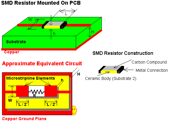
The effective substrate height is the sum of the PCB height H and the component height h. However the permittivity of each material is different. It can be shown that the composite effective permittivity €T can be determined to be
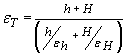
A derivation for €T can be found at the following link Composite Permittivity
Return to A Component Universe
or return to Kaleidoscope Comms